What happens to the log (concentration) vs response curve of a drug in the presence of a competitive antagonist? Assuming that the agonist and the antagonist are in equilibrium with the receptor-binding site, we will observe a parallel shift in the agonist concentration response curve. We can estimate the proportion of agonist and antagonist bound to the receptors by the concentration of the agonist and antagonist and by their affinities for the receptor as follows:

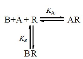Under the laws of Mass Action, we can derive the following relationship:

Where and are the dissociation equilibrium constants for the binding of A and B respectively with the receptor R.

We can rewrite these equations in terms of proportion of receptors that are either free () or occupied by either ligand A ( ) or antagonist B ( ):

                                                                         (1)

                                                                       (2)

We can thus also write the following about the state of an individual receptor, which is either in the free or occupied state as follows:

                                                              (3)

Since we are interested in , we can use eq 1 and 2 to substitute for and in equation 3 as follows:

This relationship expressed how is dependent on the concentrations of A and B and is known as the Gaddum equation named after J. H. Gaddum. In the above equation, if [B] is set to zero, we end up with the Hill-Langmuir equation.

A key assumption of this equation and the effect of a competitive antagonist on an agonists’ response is that response is directly proportional to receptor occupancy. In other words, response elicited by a proportion of receptors is similar in the presence and absence of an antagonist so long as similar proportions of receptors are occupied under both conditions.

Therefore, Gaddum and Schild show that is the same in two situations where a certain response, say 60% of elicited in the presence of an agonist [A] acting alone, and then by a concentration r[A] when the agonist is applied in the presence of the antagonist where r is the concentration ratio. This can be written as:

If the expressions on the right and the left are to take the same value, the following equality must hold:

This is the Schild equation which was first applied to the study of competitive antagonism by H. O. Schild in 1949. This equation can also be applied to models more complicated than the two-state schemes depicted here. In this post, the similar derivation is show for the del Castillo-Katz scheme. It should also be noted that the value of r is constant for a given value of [B] and regardless of the agonist used and it’s concentration assuming that the agonist and the antagonist bind to the same receptor.

The above equation can also often be reported in logarithmic scale as follows:

or

This can be plotted as a straight line with a slope of unity and the x-intercept provides an estimate of

If the agonist ratio r = 2, then the above equation can be rewritten as:

Therefore if the Schild’s relationship holds then,

Thus in summary, the Gaddum and Schild’s equations show us that the action of an antagonist can be surmounted by sufficient increase in the agonist concentration. The agonist response curve is shifted to the right in a parallel manner in the presence of a competitive antagonist and the magnitude of the right shift is expressed by the agonist concentration ratio r.

The second tab in the shiny app featured below serves to highlight the observed changes in a drug’s concentration response curve with increasing concentration of an antagonist [B]. We can see a right shift in the EC50 upon increasing concentration of [B]. The graphic below also highlights the relationship between the observed changes in apparent Ki with changes in EC50. As the amount of receptor occupancy increases in the x-axis, we would expect to see a concomitant increase in Ki of an antagonist as expected. Furthermore, small changes in EC50 can have dramatic effects on the Ki especially at low receptor occupancy when [L] < EC50.