
At work, quantification of differential gene expression is undertaken using real time RT-PCR. The technology generates a quantitative end point threshold (Ct) value defined as the threshold cycle where the fluorescent signal of the reporter dye crosses an arbitrarily placed threshold. The threshold is usually placed in the exponential phase of the PCR amplification cycle and is inversely related to the quantity of the amplicon being amplified. The following guidelines review some basic concepts of qPCR data analysis using delta delta Ct with discussions on selecting housekeeping gene and replicate analysis and data reporting. The post is intended for those users who are already familiar with the technology and have a working knowledge of the basics of qPCR.
There are usually several means of reporting real time PCR data whereby the gene expression levels could either be reported in absolute or relative expression terms. Absolute expression quantification would provide an exact copy number following interpolation of the Ct values from a standard curve and the data will normally be presented as number of copies of gene per cell or per unit mass. Relative quantification, on the other hand, provides the gene expression data relative to an internal control. Due to the difficulties associated with generating a robust standard curve for conducting absolute quantification, particularly when analyzing multiple genes, relative gene expression techniques are often utilized to simply report fold changes in gene expression as a result of an experimental treatment, thus obviating the need for determining standard curves.
Comparative Ct (ΔΔCt)
There are various ways to analyze gene expression using the relative gene expression method but a key assumption here is that the amplification efficiency of both genes tested should be the same. The comparative method reports the relative expression of the gene of interest normalized against a reference gene. Methods such as the ‘efficiency correction’ method and the ‘sigmoidal curve fitting’ methods attempt to fit the experimental data to models that predict PCR efficiency and provide an estimate of the initial copy number of the amplicon. The comparative Ct method makes an assumption that the PCR efficiency is close to 1 and that the efficiency of the target gene is similar to that of the reference gene. The disadvantage of this method, of course, is that if the efficiencies are not equal then the PCR conditions need to be further optimized. Furthermore, determining the PCR efficiencies is impractical when profiling many hundreds of genes by real-time PCR. On way to get around this problem is to approximate PCR efficiency by comparing the shape of the amplification curves. This should be done only on logarithmic PCR amplification plots and not the linear plots. Primers sets that yield a near identical shape of the amplification curves will be expected to have similar PCR efficiencies.
The final fold change in gene expression can then be calculated using the formula 2-ΔΔCt where expression levels can be compared between treated vs control groups where both the treated and the control groups are also related to an internal reference gene.
In other words:
ΔΔCt = ΔCt (treatment) – ΔCt (control) where,
ΔCt (treatment) = Ct(target gene, treatment sample) – Ct(reference gene, treatment sample) and
ΔCt (control) = Ct(target gene, control sample) – Ct(reference gene, control sample), thus
ΔΔCt = (Ct(target gene, treatment sample) – Ct(reference gene, treatment sample)) – (Ct(target gene, control sample) – Ct(reference gene, control sample))
where,
Ct(target gene, treatment sample) = Ct value of gene of interest in treated samples
Ct(reference gene, treatment sample) = Ct value of housekeeping gene in treated sample
Ct(target gene, control sample) = Ct value of gene of interest in control (calibrator) sample
Ct(reference gene, control sample) = Ct value of housekeeping gene in control (calibrator) sample
We can then calculate the relative expression of target gene in our treated sample relative to the untreated sample by calculating 2-ΔΔCt.
Let’s illustrate this with an example,
| Sample | Gene | Mean Ct |
| Control (calibrator) | GOI | 27.30 |
| Control (calibrator) | HSKG | 24.18 |
| Treatment | GOI | 21.98 |
| Treatment | HSKG | 23.78 |
ΔΔCt = ((21.98 – 23.78) – (27.30 – 24.18))
ΔΔCt = (-1.8) – (3.12)
ΔΔCt = -4.92
2-ΔΔCt = 2-(-4.92) = 30.27
Thus the expression of our gene of interest has increased by ~30 times in our treated sample versus our untreated sample.
There is often confusion around the exact order of subtraction, but consistency is the key. So as long as we subtract treated from control or reference gene from control gene, then the value of ΔΔCt will always be the same except for the sign. Take the following examples:
ΔControl vs ΔTreated
ΔΔCt = (Ct(target gene, control) – Ct(reference gene, control)) – (Ct(target gene, treatment sample) – Ct(reference gene, treatment sample))
ΔΔCt = ((27.3 – 24.18) – (21.98 – 23.78))
ΔΔCt = 4.92
ΔΔCt = (Ct(reference gene, treatment sample) – Ct(target gene, treatment sample)) – (Ct(reference gene, control sample) – Ct(target gene, control sample))
ΔΔCt = ((23.78 – 21.98) – (24.18 – 27.3))
ΔΔCt = 4.92
ΔΔCt = (Ct(reference gene, control sample) – Ct(target gene, control sample)) – (Ct(reference gene, treatment sample) – Ct(target gene, treatment sample))
ΔΔCt = ((24.18 – 27.3) – (23.78 – 21.98))
ΔΔCt = -4.92
ΔΔCt = (Ct(target gene, treatment sample) – Ct(reference gene, treatment sample)) – (Ct(target gene, control sample) – Ct(reference gene, control sample))
ΔΔCt = ((21.98– 23.78) – (27.30 – 24.18))
ΔΔCt = -4.92
Δ Reference gene vs Δ Target gene
ΔΔCt = (Ct(target gene, control sample) – Ct(target gene, treatment sample)) – (Ct(reference gene, control sample) – Ct(reference gene, treated sample))
ΔΔCt = ((27.30 – 21.98) – (24.18 – 23.78))
ΔΔCt = 4.92
ΔΔCt = (Ct(reference gene, treatment sample) – Ct(reference gene, control sample)) – (Ct(target gene, treatment sample) – Ct(target gene, control sample))
ΔΔCt = ((23.78 – 24.18) – (21.98 – 27.3))
ΔΔCt = 4.92
ΔΔCt = (Ct(reference gene, control sample) – Ct(reference gene, treatment sample)) – (Ct(target gene, control sample) – Ct(target gene, treatment sample))
ΔΔCt = ((24.18 – 23.78) – (27.30 – 21.98))
ΔΔCt = -4.92
ΔΔCt = (Ct(target gene, treatment sample) – Ct(target gene, control sample)) – (Ct(reference gene, treatment sample) – Ct(reference gene, control sample))
ΔΔCt = ((21.98 – 27.30) – (23.78 – 24.18))
ΔΔCt = -4.92
The ratio of target gene to reference gene in each sample is therefore defined as 2Ct(target gene)/2Ct(reference gene), which can be rewritten as 2(Ct(target gene) – Ct(reference gene))
The ratio between the target gene to reference gene between our treated and untreated control samples can be written as:

Which is the same as
2(Ct(target gene, control sample) – Ct(reference gene, control sample)) – (Ct(target gene, treatment sample) – Ct(reference gene, treatment sample))
Determination of PCR efficiency
The general rule for determining PCR efficiency of either your gene of interest and/or your housekeeping gene is to generate Ct values on serially diluted cDNA template. Alternatively, you could also use serial dilutions of the total RNA as a template and the subsequent PCR efficiency calculations would take into account the efficiency of both the reverse transcription and the PCR amplification steps. PCR efficiency (E) can be calculated by plotting the Ct value (y-axis) against the log cDNA serial dilution (x – axis) across a 10-log concentration range (Figure 1). The slope of the line generated upon regressing across the Ct values should allow you to calculate the PCR efficiency using the following equation: , where m is the slope of the line and E is the efficiency. A slope close to -3.322 indicates 100% efficiency, or E = 2, which can then be incorporated into the formula for calculating the concentration as follows (E)-ΔΔCt. A rough guide is to work with primer sets which give, at least, greater than 95% efficiency and that the differences in efficiency between two genes should be within 10% of each other (i.e. 1.8 x – 2.2 x).
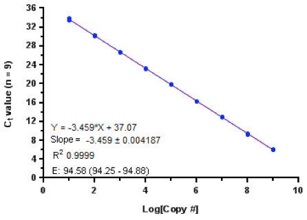
Figure 1: Standard curve derived from plasmid DNA template spanning across a 9-log concentration range performed in 9 replicates. A linear regression with an R2 of 0.9999 is used to derive a slope of -3.459 which yields a 95% efficiency of replication
Selecting the right reference gene
Since qPCR experiments generally measure sample quantity rather than concentration, the measurements are subject to sample size based variation and various normalization methods are available in order to compensate for this. The most widely used method for normalization is to normalize against a reference gene. This allows one to not only normalize against variations in loading amount, but also for variations in sample extraction, RT efficiency and RNA quality. A good housekeeping gene should, ideally, have a stable expression amongst the samples tested and its expression levels should be unaffected by the experimental treatment being examined. Another method that is often employed is to normalize the expression of test gene by the quantities of total RNA. A gene that reflects the lowest intra and inter sample standard deviation will strongly correlate with the amount of total RNA, in which case we would be justified in normalizing the expression levels to the amount of total RNA directly. This method, however, does not take into account the ratio of mRNA to total RNA in the samples or the quality of RNA being evaluated. Alternatively, an analysis of variance based approach can be applied to identify the best housekeeping gene with which to normalize the expression levels of our gene of interest. This approach is expounded in the tool Normfinder (Andersen et al. (2004) Cancer Res. Aug 1; 64 (15): 5245-50). Normfinder is usually applied to a selected panel of candidate reference genes which is analyzed in a set of representative samples. A global average expression of all genes is then calculated in all of the samples tested and a standard deviation for each of the candidate reference genes is calculated. An intragroup standard deviation calculates the variation in the expression of the genes within the various different treatment groups, while the intergroup standard deviation calculates the differential expression of each of the candidate genes over all the treatment groups. The ideal candidate gene is then determined as the one with low intragroup variation, as well as, the lowest intergroup variation. A manual inspection of the data is often necessary in order to remove from the analysis any obvious gene candidates which are regulated by the treatment conditions or are inherently unstable. The analysis should then be repeated with this set of genes deleted. An ‘accumulated standard deviation’ can often be calculated by certain programs to allow the use of multiple housekeeping genes. Accumulated standard deviation is often lower than that obtained from a single reference gene, as random variance of each gene serves to cancel each other out; however, it can often be quite tedious to measure multiple genes which make this approach a tradeoff between the amount of effort required to screen multiple genes and the improvement in accumulated standard deviation achieved. An interesting note to keep in mind is that if your standard deviation of technical repeats is rarely less than 0.1 Ct then including housekeeping genes with accumulated standard deviations of less than 0.1 will not offer a significant improvement in the quality of the data. In this case, we would want to ensure that we eliminate housekeeping candidate genes with standard deviation of greater than 0.1 cycles. An excel plug in for Normfinder can be found here: http://moma.dk/normfinder-software.
Another older algorithm for calculating the best housekeeping gene is called geNorm (Vandesompele et al. (2002) Genome Biology (3)). This essentially uses the same data input as the Normfinder algorithm, however, it does not calculate inter group variation. geNorm calculates paired expression values in all of the representative study samples and then iteratively eliminates the genes that display the highest variation relative to all the other genes in the analysis. A final pair of genes is returned by geNorm which show the highest correlation and lowest variation (M-value) between samples. The problem with M values in geNorm is that the variance for candidate genes can be calculated based on unequal sample sizes, which makes it difficult to compare across genes, unlike in ANOVA analysis used in Normfinder. I prefer to use Normfinder but for those interested, this is a plug in for geNorm available here: https://genorm.cmgg.be/
Analysis of replicate data and error propagation
In qPCR experiments, a common source of confusion arises in the propagation of errors. This becomes particularly important in absolute PCR analysis where the errors of the test samples are additive with the errors in the generation of the standard curve and one has to take into account the various normalization steps during data preprocessing. In comparative Ct analysis, where typically two to four PCR replicates are run per cDNA sample, error propagation is slightly more intuitive. Firstly, it is important to realize that, whereas, the gene expression levels within a population of cells is log normally distributed (Bengtsson, M. et. al., (2005) Genome Research 15:1388–1392; Raj A., et. al., (2006) PLoS Biol 4(10); Limpert E., at. al., (2001) BioScience 51(5)), the derived Ct values obtained from qPCR experiments are normally distributed; therefore, the replicate Ct values can be averaged using arithmetic mean in order to calculate the average fold change in expression. If, however, we use the concentration values (i.e. 2Ct), then we may wish to use geometric mean to calculate average of replicates. Likewise, it would, therefore, be correct to calculate the standard deviation or standard error of the replicate Ct values first and report these errors in the concentration bar plots upon log transformation. Calculating the standard deviation of the concentration values and or ratios of concentrations for subsequent depiction in a bar plot is not correct as these values are log normally distributed. In other words, properly calculated error bars should be asymmetric on the linear x scale.
The error in ΔΔCt experiments is additive of the error of (target gene, control sample) + (reference gene, control sample) + (target gene, treatment sample) + (reference gene, treatment sample). Based on the laws of error propagation for additions and subtractions, the type of additive error in our qPCR experiments can usually be propagated using where and are standard errors of control and treatment samples.
Another source of confusion often arises when reporting fold changes upon down regulation of genes. In other words, if in our ΔΔCt experiments, the first ΔCt value is greater than the second ΔCt value, then the outcome of 2-ΔΔCt will be < 1 implying a reduction in gene expression due to treatment. Here, depicting a bar plot with ΔΔCt values can be a bit misleading as a value of 2 would denote 2-fold up regulation but a ΔΔCt of 0.5 would then appear misleading as it might suggest a half a fold increase, whereas, a ΔΔCt of 0.5 actually denote a 2-fold change in the negative direction or 2-1/ΔΔCt.Therefore, when depicting gene down regulation (0 < ΔΔCt < 1), it’s best to plot the results as fold-changes in gene expression by taking the negative inverse of 2-ΔΔCt.
Most folks prefer to report these changes in gene expression data as a bar plot on a continuous y-axis. I find this slightly troublesome as it implies that where y = 0, the fold change in gene expression (2x) is equal to 0 and we can’t really define log100 when we try to solve for x. Alternatively, we can log2 transform the fold changes in gene expression data and report this scale on the y-axis (Figure 2). This means that the value of 1 or -1 on the y-axis corresponds to 2-fold change in the positive and negative direction respectively and 0 indicates 20 = 1 or no change in gene expression.
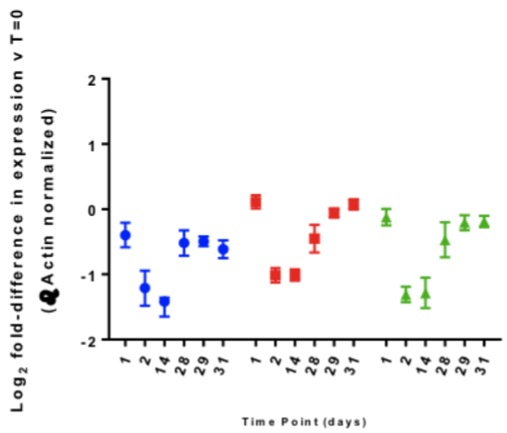
Figure 2: Fold Differences in gene A (blue), gene B (red) and gene C (green) for all donors over all time points, including +/- range
