
In biological testing, we often encounter statistical analysis that shows comparison between groups of data sets. A p-value is often used to show the strength of the evidence to support a difference in means between those two groups of data. These p-values are the bread and butter in both pair wise and multiple comparison hypothesis testing.
So let me ask you this question, if you saw two groups of data shown to be statistically different with a p-value of say, 0.05, would you agree that the difference between the two groups is indeed significant?
The most common response to this question would be, that there is only a 5% chance (p = 0.05) of observing this degree of difference between the two groups, if this difference were not a real effect. In statistical terminology, the probability of committing a type I error in this instance is 5%. So, yes, the popular opinion would be that the difference is real.
This answer, somewhat contrary to what we’ve all been taught in school, is false. Well, not entirely true at the very least, let me explain –
In significance testing, the p-value, on its own does not give a complete understanding. The true answer relies on another factor called the Positive Predictive Value (PPV) of a significant p-value. In other words, the PPV reflects the probability of a significant p-value occurring that arises due to a real effect. This is a somewhat intractable concept, which perhaps will become clearer with the schematic that follows below. Conversely then, the probability of observing significant p-value that arises due to a null effect is defined as the False Discovery Rate (FDR), which is more akin to the original question we were trying to ask.
Let’s take an example – say we carry out a test to study the expression of a particular disease biomarker in 100 randomly chosen patients.
Now also, for the purpose of this exercise, let’s say that we already know that 20% of those patients have the disease in question and, therefore, they should register as true positives for the biomarker.
Upon testing, we would expect to see 20 tests that register a real result and 80 tests that register a false result under ideal conditions. But, of course, this outcome represents the ideal condition, where our testing method is 100% efficient. What if the biological assay we used for conducting this test was only 60% efficient? In other words, what if the ‘power’ of the assay used to detect this biomarker was only was 60% for a given ‘effect size’. Now if we run our analysis again and set our alpha level to 5%, we would see the following:
Of the 100 tests conducted, we would expect 20 tests to show a real effect and 80 tests to show a null effect, because of the prior knowledge we have about the percentage of diseased population in this dataset. But, of course, since the power of our biological assay is only 60%, we expect that only 0.60 * 20 = 12 cases will be detected as true positives, with the remaining 8 being dismissed as non-significant false-negatives. Meanwhile, of the 80 tests that showed a null effect, we would expect to see 0.05 * 80 = 4 p-values that are significant by chance alone (false positives) and 76 of the remaining would be classified as non-significant true negatives.
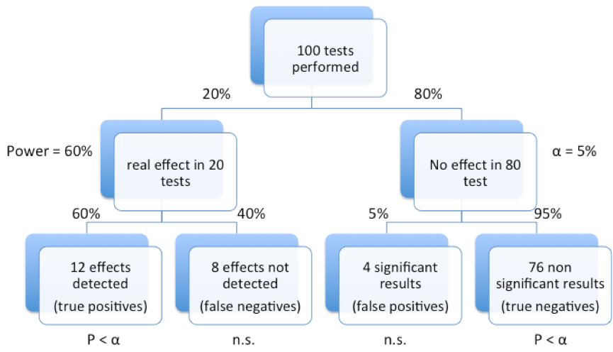
Figure 1. Tree diagram illustrating false discovery rates in significance testing.
So, of the (12 + 4) positive outcomes, only 12 are actual positives, therefore, our FDR is 4/(12 + 4) = 0.25 or 25% (1 in 4) which is substantially larger than the 5% (1 in 20) set by our significance threshold. Likewise, our PPV is 12/(12 + 4) = 0.75 or 75%.
So, using a test with higher power will inevitably increase the number of true positives, but in experiments with small effect sizes, the size requirements for observing a 90% or 99% power can be prohibitive (discussion on power calculations is beyond the scope of this article). Likewise, using a more stringent significance threshold (i.e. greater than 95%) would equally decrease the number of false positives. In fact, in our example above, by simply changing the significance threshold from 95% to 99% we would decrease our FDR to 0.06 or (1 in 16), a figure much closer to the initially desired 5% significance.
In our example where an assay with 60% power was chosen to detect the disease biomarker, one can easily see how an FDR of 1 in 4 will hardly qualify as a ‘significant’ result, with only a 1 in 4 chance of reproducibility. It is, therefore, not surprising that most published research findings are false, as John P. A. Ioannidis reminded us in his now famous paper, Why Most Published Research Findings Are False [1].
The ‘back of the envelope’ analysis presented above bears a formal similarity to a Bayesian analysis, but perhaps can be, more simplistically, thought of as a conditioned probability problem [2]. More formally, Bayes’ rule is defined as:

where, A and B are related events and the conditional probability of an event B given A has occurred is:

In our example above, if we define the ‘+’ and ‘-’ as the events that define the result of our biomarker test as positive or negative respectively, and B and Bc as the event that the subject of the test either has or does not have the biomarker respectively, then the following definitions hold:
The sensitivity (Power) of a test is defined as the probability of a test being positive given that the subject actually has the biomarker present, P(+|B)
The specificity (1 – alpha) (true negative) of a test is then defined as the probability of a test being negative given that the subject does not have the biomarker present, P(-|Bc)
The positive predictive value in this case, is the probability that the subject has the biomarker given that the test is positive, P(B|+)
The negative predictive value, conversely can be defined as the probability of a test being negative given that the subject does not have the biomarker, P(Bc|-)
Finally, the prior probability, which was defined as the prevalence of the disease in our population is defined as P(B).
So, in our example previously, where we defined the biomarker test to have a sensitivity P(+|B) of 0.60% and a specificity P(-|Bc) of 95% with 20% prevalence P(B), we can define the positive predictive value P(B|+) as follows:

or

thus 
= 0.75
Therefore, the FDR is 1 – 0.75 = 0.25 or 1 in 4 as shown previously.
A similar result can be obtained by simulating the above example using some R code. Two groups (group 1, group 2) of random observations are generated, a 1000 times over, with specified means of 0 and 1 respectively and having the same standard deviation. Each group consists of 16 observations where the observations are normally distributed, and therefore, the assumptions of t-tests are valid.
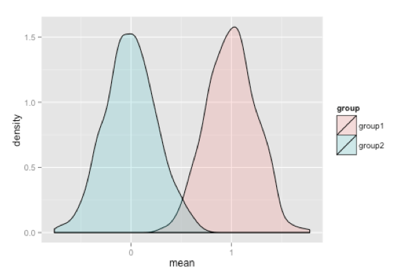
Figure 2. Distribution of simulated means of 16 normally distributed observations between control group 1 and treatment group 2 that differ by 1 s.d.
The t-distribution of the difference in the means of the 1000-simulated tests shows that the difference of mean is close to 1 as seen in Figure 3b. The distribution of the 1000 p-values generated is shown in Figure 3a where the number of p-values that are less than or equal to 0.05 is 776 out of a 1000 tests or 78%. A look at the power calculation for this t-test is 78% (see R code), which is also in keeping with our simulated experiment. In other words, 78% of the simulated t-tests give the correct result.
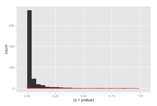

Figure 3. Distribution of a 1000 simulated t-tests showing (A) the distribution of 1000 p-values, with 78% equal to or less than 0.05 and (B) showing the distribution of the difference between means of the 16 observations between the two groups
The effect on the number of significant p-values is immediately apparent were we to decrease the power of the test by reducing the number of observations in each simulation to, say 6. The power of the test in this instance would change to 35%. If we rerun the 1000 simulations with n = 6, then we can see in Fig 4 that the number of p-values that are significant changes to 336 out of a 1000, which is 33.6%.
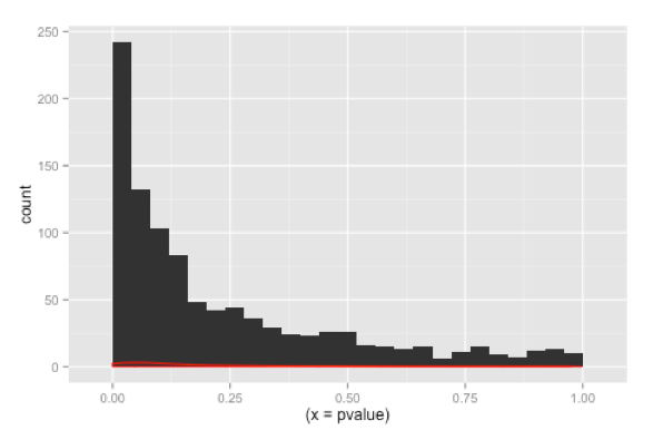
Figure 4. Distribution of 1000 p-values, with n = 6, instead of 16, showing 336 p-values (33.6 %) to be significant which is close to the calculated power of 35%.
In our simulated example, of the 1000 simulations, we would expect 5% to be false positives (p =< 0.05), i.e. 50 false positives and we know that there are 78% true positives, i.e. 780. If we consider a prevalence of 20% for our positive test, then, we can expect 0.8(50) + 0.2(780) = 40 + 156 = 196 positive tests of which 50 are false positives. Therefore, if a positive test is observed, the probability of it being a false positive is 0.8(50)/196 = 0.204 = 20.4% which is the False Discovery Rate.
In both the ‘Frequentist’ and ‘Bayesian’ approaches to tackling this type of analysis presented here, what becomes clear is that relying on a p = 0.05 as a standard cut off point for testing biological significance, will very likely lead us to claim a real effect when there is none (i.e. commit a type I error). Underpowered studies will, therefore, significantly contribute towards seeing a higher FDR and inflation of ‘effect sizes’. Interestingly, in such instances, quoting a 95% confidence interval will not necessarily convey any more meaning about the true FDR of the assay. In these cases, adopting a more stringent cutoff such as p < 0.001 would perhaps be wiser to avoid the risk of making a claim that can’t be reproducibly substantiated.
The R code for the simulation experiment and the figures can be found at this link: pvalue/pvalues.R
References
1. Ioannidis JP a (2005) Why most published research findings are false. PLoS Med 2:0696–0701. doi: 10.1371/journal.pmed.0020124
2. Colquhoun D (2014) An investigation of the false discovery rate and the misinterpretation of P values. R Soc Open Sci 1–15. doi: 10.1098/rsos.140216
